随机种子 1 2 3 4 5 6 7 8 9 10 11 12 def seed_everything (seed ): torch.manual_seed(seed) torch.cuda.manual_seed(seed) torch.cuda.manual_seed_all(seed) torch.backends.cudnn.benchmark = False torch.backends.cudnn.deterministic = True random.seed(seed) np.random.seed(seed) os.environ['PYTHONHASHSEED' ] = str (seed) seed_everything(0 )
数据部分 在引用路径时,\被识别成转义字符怎么办? 在前面加r
1 2 path = r"C:\Users\a'diao\Desktop\深度学习项目复试\第四节\food_classification\food-11\training\labeled"
读取文件 1 2 3 4 5 6 7 8 9 10 11 12 13 14 15 16 17 18 19 20 21 22 23 24 25 26 27 HW = 224 def read_file (path ): for i in tqdm(range (11 )): file_dir = path + "/%02d" %i file_list = os.listdir(file_dir) xi =np.zeros((len (file_list),HW,HW,3 ),dtype=np.uint8) yi = np.zeros(len (file_list), dtype=np.uint8) for j,name in enumerate (file_list): img_path = os.path.join(file_dir,name) img = Image.open (img_path) img = img.resize((HW,HW)) xi[j, ...] = img yi[j] = i if i == 0 : X = xi Y = yi else : X = np.concatenate((X, xi), axis=0 ) Y = np.concatenate((Y, yi), axis=0 ) print ("读到了%d个数据" % len (Y)) return X, Y
listdir()函数 输入参数为文件夹的路径,读取这个文件夹的全部文件名并以list的格式返回
例如:
1 2 3 4 5 6 ./data/labeled_data/00/ ├─ apple_01.jpg # 有效图像 ├─ apple_02.png # 有效图像 ├─ temp.txt # 非图像文件 ├─ sub_dir/ # 子文件夹 └─ .DS_Store # 系统隐藏文件(mac)/ desktop.ini(Windows)
返回结果:[‘apple_01.jpg’, ‘apple_02.png’, ‘temp.txt’, ‘sub_dir’, ‘.DS_Store’]
甲是干什么的? 由于乙,读到的x是图像名称,y是第i个文件夹即第i类。最后把数据按列拼在一起
数据增广 训练的时候需要增广,但验证和测试的时候并不需要
1 2 3 4 5 6 7 8 9 10 11 12 13 14 15 train_transform = transforms.Compose( [ transforms.ToPILImage(), transforms.RandomResizedCrop(224 ), transforms.RandomRotation(50 ), transforms.ToTensor() ] ) val_transform = transforms.Compose( [ transforms.ToPILImage(), transforms.ToTensor() ] )
加载数据集 1 2 3 4 5 6 7 train_path = r"C:\Users\a'diao\Desktop\深度学习项目复试\第四节\food_classification\food-11_sample\training\labeled" val_path = r"C:\Users\a'diao\Desktop\深度学习项目复试\第四节\food_classification\food-11_sample\validation" train_set = food_Dataset(train_path,"train" ) val_set = food_Dataset(val_path,"val" ) train_loader = DataLoader(train_set,batch_size=4 ,shuffle=True ) val_loader = DataLoader(val_set,batch_size=4 ,shuffle=True )
train_set、train_loader分别有什么作用 train_set:实例化对象,把指定路径下的所有图像 + 标签,封装成 PyTorch 的Dataset对象(可以理解为 “数据手册”,记录了每一张图的路径、标签,以及如何读取它);
train_loader:我们已经有了train_set,能够按索引返回图片和标签(即X和Y),但这并不方便我们操作,而DataLoader在这里的作用就是成批的录入数据(batch)和打乱顺序(shuffle)
模型部分 1 2 3 4 5 6 7 8 9 10 11 12 13 14 15 16 17 18 19 20 21 22 23 24 25 26 27 28 29 30 31 32 33 34 35 36 37 38 39 40 41 42 43 44 45 46 class myModel (nn.Module): def __init__ (self,num_cls ): super (myModel,self ).__init__() self .conv1 = nn.Conv2d(3 ,64 ,3 ,1 ,1 ) self .bn = nn.BatchNorm2d(64 ) self .relu = nn.ReLU() self .pool1 = nn.MaxPool2d(2 ) self .layer1 = nn.Sequential( nn.Conv2d(64 , 128 , 3 , 1 , 1 ), nn.BatchNorm2d(128 ), nn.ReLU(), nn.MaxPool2d(2 ) ) self .layer2 = nn.Sequential( nn.Conv2d(128 , 256 , 3 , 1 , 1 ), nn.BatchNorm2d(256 ), nn.ReLU(), nn.MaxPool2d(2 ) ) self .layer3 = nn.Sequential( nn.Conv2d(256 , 512 , 3 , 1 , 1 ), nn.BatchNorm2d(512 ), nn.ReLU(), nn.MaxPool2d(2 ) ) self .pool2 = nn.MaxPool2d(2 ) self .fc1 = nn.Linear(25088 , 1000 ) self .relu2 = nn.ReLU() self .fc2 = nn.Linear(1000 , num_cls) def forward (self,x ): x = self .conv1(x) x = self .bn(x) x = self .relu(x) x = self .pool1(x) x = self .layer1(x) x = self .layer2(x) x = self .layer3(x) x = self .pool2(x) x = x.view(x.size()[0 ],-1 ) x = self .fc1(x) x = self .relu2(x) x = self .fc2(x) return x
SGD和Adam和AdamW的区别 SGD:随机梯度下降。只会朝着梯度的反方向移动。
Adam:自适应矩估计。会同时参照当前梯度和以前的梯度,a* old+(1-a)* new。相比于SGD的改进点有两个:梯度和学习率
AdamW:在Adam上加一个权重衰减,loss+y* W**2
迁移学习 借用大佬的模型,让我们的模型一开始就具有特征提取的能力,最后换一下探测头(即最后分多少类),这样效果会比用自己的模型好很多。
另外,要注意pretrained这个参数,为True时既使用参数又使用模型,为FALSE时只使用模型。当然,为True时效果更好。
这也解释了为什么我们要使用别人的架构,只有使用了别人的架构才能使用它们的参数。
线性和微调 线性就是完全相信大佬的模型,通过设置梯度为零的方式保持参数不变。
微调就是调用大佬的模型后,仍然会改变它的参数。
一般都用微调。
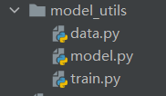
咋样让代码变得简单呢 首先,只用main函数,在main函数里面调用别的代码:
1 2 3 from model_utils.model import initialize_modelfrom model_utils.train import train_valfrom model_utils.data import getDataLoader
不过,使用这种方法时,非main函数要加一段代码。这里的__main__并非main函数,而是指调用的是当前模块
1 2 3 4 5 6 7 8 if __name__ == '__main__' : filepath = '../food-11_sample' train_loader = getDataLoader(filepath, 'train' , 8 ) for i in range (3 ): samplePlot(train_loader, True , isbat=False , ori=True ) val_loader = getDataLoader(filepath, 'val' , 8 ) for i in range (100 ): samplePlot(val_loader, True , isbat=False , ori=True )
核心作用是让 Python 模块中的特定代码块仅在该模块被直接运行时执行,而在被其他模块导入复用(函数 / 类等)时不执行,从而实现复用逻辑与直接运行逻辑的隔离 。
其次,运行时把超参数改成字典
1 2 3 4 5 6 7 8 9 10 11 12 13 14 15 16 17 18 19 20 21 22 23 24 25 26 27 28 29 30 31 32 33 34 35 36 lr = 0.001 loss = nn.CrossEntropyLoss() optimizer = torch.optim.AdamW(model.parameters(), lr=lr, weight_decay=1e-4 ) device = "cuda" if torch.cuda.is_available() else "cpu" epoch = 3 save_path = "model_save/best_model.pth" thres = 0.99 train_val(model, train_loader, val_loader, no_label_loader, device, epoch, optimizer, loss, thres, save_path) trainpara = { "model" : model, 'train_loader' : train_loader, 'val_loader' : val_loader, 'no_label_Loader' : no_label_Loader, 'optimizer' : optimizer, 'batchSize' : batchSize, 'loss' : loss, 'epoch' : epoch, 'device' : device, 'save_path' : save_path, 'save_acc' : True , 'max_acc' : 0.5 , 'val_epoch' : 1 , 'acc_thres' : 0.7 , 'conf_thres' : 0.99 , 'do_semi' : True , "pre_path" : None } if __name__ == '__main__' : train_val(trainpara)
训练函数 1 2 3 4 5 6 7 8 9 10 11 12 13 14 15 16 17 18 19 20 21 22 23 24 25 26 27 28 29 30 31 32 33 34 35 36 37 38 39 40 41 42 43 44 45 46 47 48 49 50 51 52 53 54 55 56 57 58 59 60 61 62 63 64 65 66 67 68 69 70 71 72 73 74 75 76 def train_val (model, train_loader, val_loader, no_label_loader, device, epochs, optimizer, loss, thres, save_path ): model = model.to(device) semi_loader = None plt_train_loss = [] plt_val_loss = [] plt_train_acc = [] plt_val_acc = [] max_acc = 0.0 for epoch in range (epochs): train_loss = 0.0 val_loss = 0.0 train_acc = 0.0 val_acc = 0.0 semi_loss = 0.0 semi_acc = 0.0 start_time = time.time() model.train() for batch_x, batch_y in train_loader: x, target = batch_x.to(device), batch_y.to(device) pred = model(x) train_bat_loss = loss(pred, target) train_bat_loss.backward() optimizer.step() optimizer.zero_grad() train_loss += train_bat_loss.cpu().item() train_acc += np.sum (np.argmax(pred.detach().cpu().numpy(), axis=1 ) == target.cpu().numpy()) plt_train_loss.append(train_loss / train_loader.__len__()) plt_train_acc.append(train_acc/train_loader.dataset.__len__()) if semi_loader!= None : for batch_x, batch_y in semi_loader: x, target = batch_x.to(device), batch_y.to(device) pred = model(x) semi_bat_loss = loss(pred, target) semi_bat_loss.backward() optimizer.step() optimizer.zero_grad() semi_loss += train_bat_loss.cpu().item() semi_acc += np.sum (np.argmax(pred.detach().cpu().numpy(), axis=1 ) == target.cpu().numpy()) print ("半监督数据集的训练准确率为" , semi_acc/train_loader.dataset.__len__()) model.eval () with torch.no_grad(): for batch_x, batch_y in val_loader: x, target = batch_x.to(device), batch_y.to(device) pred = model(x) val_bat_loss = loss(pred, target) val_loss += val_bat_loss.cpu().item() val_acc += np.sum (np.argmax(pred.detach().cpu().numpy(), axis=1 ) == target.cpu().numpy()) plt_val_loss.append(val_loss / val_loader.dataset.__len__()) plt_val_acc.append(val_acc / val_loader.dataset.__len__()) if epoch%3 == 0 and plt_val_acc[-1 ] > 0.6 : semi_loader = get_semi_loader(no_label_loader, model, device, thres) if val_acc > max_acc: torch.save(model, save_path) max_acc = val_acc print ('[%03d/%03d] %2.2f sec(s) TrainLoss : %.6f | valLoss: %.6f Trainacc : %.6f | valacc: %.6f' % \ (epoch, epochs, time.time() - start_time, plt_train_loss[-1 ], plt_val_loss[-1 ], plt_train_acc[-1 ], plt_val_acc[-1 ]) ) plt.plot(plt_train_loss) plt.plot(plt_val_loss) plt.title("loss" ) plt.legend(["train" , "val" ]) plt.show()
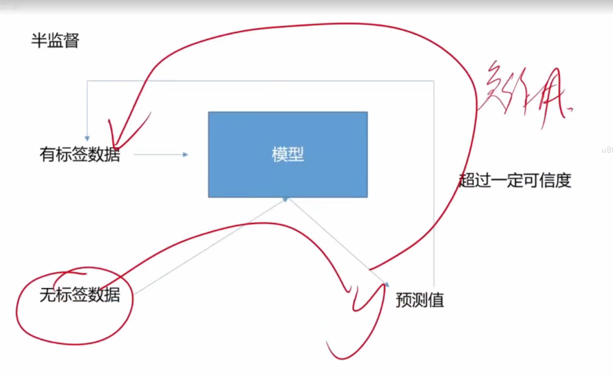
半监督学习 即在无标签的情况下,训练数据
如自训练,先学习少量有标签数据,然后自己预测无标签数据,然后把自己觉得正确率高的那部分打上标签,如此反复。
1 2 3 4 5 6 7 8 9 10 11 12 13 14 15 16 17 18 19 20 21 22 23 24 25 26 27 28 29 30 31 32 33 34 35 36 37 38 39 40 41 42 43 44 45 46 47 48 class semiDataset (Dataset ): def __init__ (self, no_label_loder, model, device, thres=0.99 ): x, y = self .get_label(no_label_loder, model, device, thres) if x == []: self .flag = False else : self .flag = True self .X = np.array(x) self .Y = torch.LongTensor(y) self .transform = train_transform def get_label (self, no_label_loder, model, device, thres ): model = model.to(device) pred_prob = [] labels = [] x = [] y = [] soft = nn.Softmax() with torch.no_grad(): for bat_x, _ in no_label_loder: bat_x = bat_x.to(device) pred = model(bat_x) pred_soft = soft(pred) pred_max, pred_value = pred_soft.max (1 ) pred_prob.extend(pred_max.cpu().numpy().tolist()) labels.extend(pred_value.cpu().numpy().tolist()) for index, prob in enumerate (pred_prob): if prob > thres: x.append(no_label_loder.dataset[index][1 ]) y.append(labels[index]) return x, y def __getitem__ (self, item ): return self .transform(self .X[item]), self .Y[item] def __len__ (self ): return len (self .X) def get_semi_loader (no_label_loder, model, device, thres ): semiset = semiDataset(no_label_loder, model, device, thres) if semiset.flag == False : return None else : semi_loader = DataLoader(semiset, batch_size=16 , shuffle=False ) return semi_loader

 微信
微信 支付宝
支付宝